Simulation Dashboard

For an elaborated example on how to interpret the Hysopt Simulation Dashboard, see Hysopt Simulation Dashboard – Example Load Profile Analysis

Introduction

The Simulation Dashboard is a post-simulation analysis tool in Hysopt that provides a pre-built analysis dashboard of the building demand. The dashboard analysis can be used as input for early-stage system sizing or for general project reporting purposes.

The dashboard enables users to:

• Analyse heating and cooling load profiles

• Identify peak loads, base loads, and simultaneity

• Support early sizing decisions for potential production systems (order of magnitude)

• Explore the potential for heat recovery and storage concepts

The Simulation Dashboard is intended as a first sizing and exploration tool. Insights gained from the dashboard should be used for selecting appropriate Hysopt templates or custom energy centre concepts, which can be further refined in more detailed Hysopt simulations.

How to Use the Simulation Dashboard

The Simulation Dashboard is a post-simulation tool and requires a completed simulation with appropriate Dashboard Measurement BCs in place. In order to correctly use the dashboard, the following workflow should be followed: defining the measurement locations, running the simulation, and opening the dashboard.

Step 1 – Place Dashboard Measurement BC

Before running a simulation, the relevant heat flows that should be input to the simulation dashboard must be defined explicitly. This is done by placing one or more Dashboard Measurement BCs in the system. In general, you want to input the full building load as input to the dashboard. This can be achieved by placing a dashboard measurement BC at the main collector.

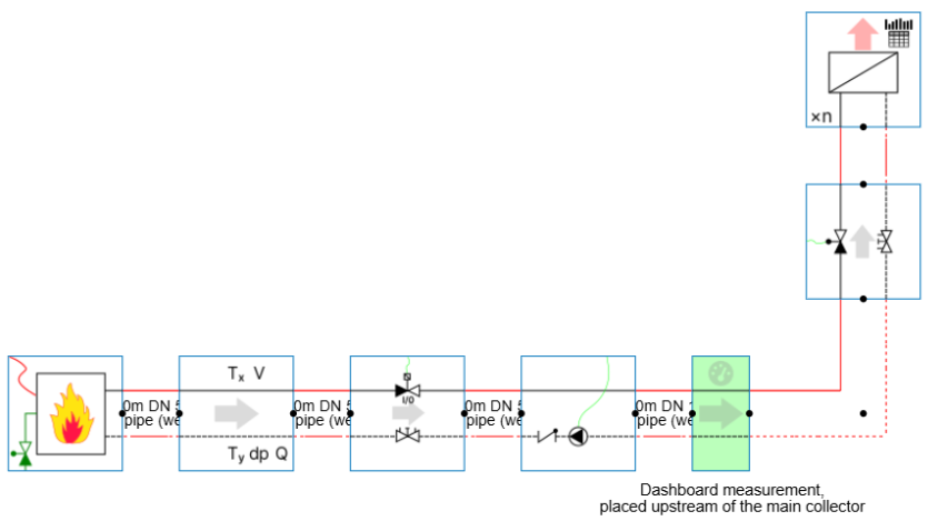
Dashboard Measurements are available under System Peripherals and are available in the heating, cooling, and changeover library. Each measurement records the heat flow at its location and provides this data to the Simulation Dashboard.

Multiple Dashboard Measurements can be used within the same model. Dashboard Measurements BCs should always be placed in parallel and positioned at locations that represent the load boundary intended for analysis. The dashboard input is calculated as the sum of all measured heat flows. Positive values are interpreted as heating demand, while negative values are interpreted as cooling demand. Heating and cooling loads are therefore always evaluated separately.

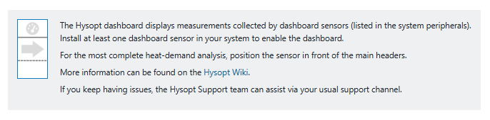
If you would forget to place any Dashboard Measurement BC in the model, the following figure will be displayed when opening the Hysopt Simulation Dashboard:

Step 2 – Run the Simulation

After the Dashboard Measurement components have been placed at the desired locations, the model can be simulated as usual. During the simulation, each measurement records its heat flow. Once the simulation has completed, the recorded data is available for post-simulation analysis. If no simulation has been run, the Simulation Dashboard cannot be used.

Step 3 – Open the Simulation Dashboard

After a successful simulation, the Simulation Dashboard can be opened using the Simulation Dashboard button located next to the Simulate button in the top ribbon bar. The simulation dashboard will be opened in a separated browser tab so that it can be placed next to the Hysopt model itself.

Simulation Dashboard Anatomy

The Simulation Dashboard is organised into three sections and is intended to be read from top to bottom, starting with general load characteristics and progressing towards more specific analyses related to heat recovery and storage. A header bar is available to manage the displayed results.

Dashboard Header bar

At the top-right of the Simulation Dashboard, a header bar provides general information about the active model, along with several dashboard control buttons.

The header includes the following elements:

• Simulation finish time:

Displays the time when the simulation was completed, and the dashboard was generated for the first time.

• Model name
  Displays the name of the model for which the results are currently shown, useful when working with multiple models or variants.

• Settings
  Opens the dashboard settings panel. This panel allows configuration of the sampling interval used for all curves in the dashboard. Note that small sampling intervals might yield long loading times.

• Print dashboard
  Allows the dashboard to be printed or exported for reporting purposes. If the dashboard does not fit well on a page, adjusting the print scaling is recommended.

• Refresh dashboard
  Updates the dashboard with the latest simulation results. This must be used after running a new simulation while the dashboard is already open with outdated simulation results.

General Energy and Load Analysis

The first analytical section of the dashboard provides a general overview of the heating and cooling behaviour of the model. This section is primarily intended for understanding overall load characteristics and for supporting early-stage system sizing decisions.

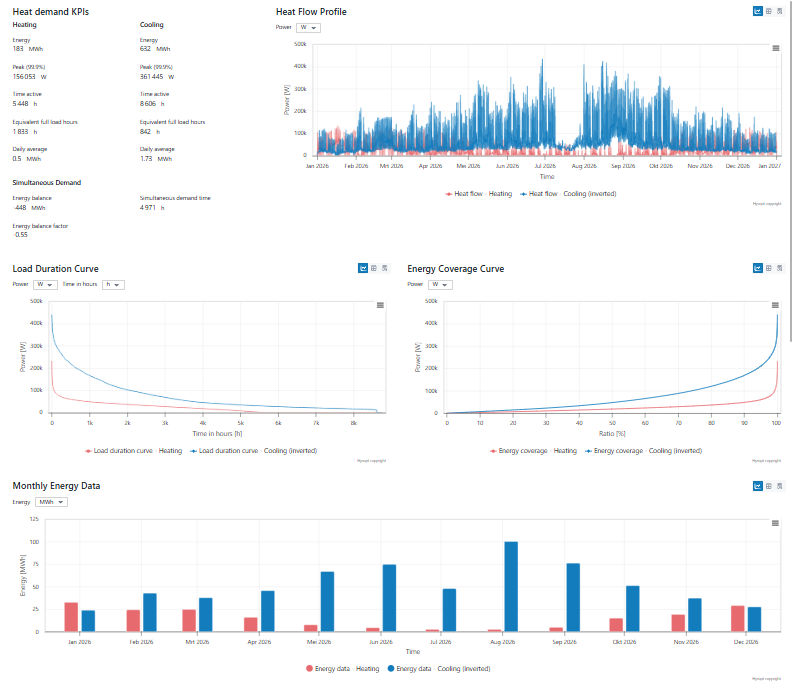
Key Performance Indicators (KPIs)

At the top of this section, a set of key performance indicators summarises the most relevant load metrics. These indicators are shown separately for heating and cooling and are complemented by metrics related to simultaneous demand.

The KPIs include:

• Energy
  The total heating or cooling energy over the simulation period.

• Peak power (99.9% energy coverage)
  The power that provides an energy coverage of 99.9%. The choice for 99.9% peak power avoids oversizing based on extreme short time-step peaks.

• Active time
  The total duration during which heating or cooling demand is present. The system is assumed to be active when above 2% of the 99.9% peak heat flow to exclude for leakage heat flows.

• Equivalent full load hours (EFLH)
  The total energy delivered by a system over a given period, divided by the design heat flow at the dashboard measurement BCs. The sum of the design heat flows is used if multiple dashboard BCs are present in the model, whilst splitting heating and cooling.

If you want to customise the applied design heat flow in the EFLH calculation, you can adjust the design heat flow for heating and cooling on the dashboard measurement BCs in your model.

• Daily average heat flow
  The daily average heating or cooling energy over the simulation period. This metric gives an intuitive idea of the amount of heat flow required for the building.

In addition, simultaneous demand is characterised using:

• Net energy balance
  The integrated difference between heating and cooling energy over the simulation period. A positive value indicates that the building has more heating demand than cooling demand. A negative value indicates that the building has more cooling demand than heating demand.

• Energy balance factor
  A normalised indicator between -1 and +1 of the net energy balance describing how well heating and cooling demands are balanced. The closer the value to zero, the more potential for energy recuperation between the heating and cooling demand. Values close to +1 or -1 indicate low potential for energy recuperation. The meaning of the energy balance factor can be intuitively understood for following three scenarios:

  • +1: Only heating demand, no cooling demand. Maximal energy imbalance with no potential for heat recovery.

  • 0: The heating demand over the simulation duration equals the cooling demand. The system is energetically speaking fully balanced. There is maximal potential for heat recovery.

  • -1: Only cooling demand, no heating demand. Maximal energy imbalance with no potential for heat recovery.

• Simultaneous demand duration
  The amount of time during which heating and cooling occur at the same time. This can indicate potential for heat recovery solutions.

Graphs

Heat Flow Profiles

Next to the KPIs, the heat flow profiles for heating and cooling are shown over time. These profiles visualise seasonal trends, base load levels, and peak demand periods. The graphs help identify when heating or cooling dominates throughout the year.

Load Duration Curves

The load duration curves display heating and cooling loads sorted from highest to lowest value. They show how long a certain load level is exceeded and are useful for identifying peak load demands and base load demands.

Energy Coverage Curves

The energy coverage curves show the share of the total annual energy demand (x-axis) that is below a given heat flow capacity (y-axis). The energy coverage curves tells what capacity is required to cover a given percentage of the total energy demand. The coverage curves support early evaluation of hybrid system concepts by highlighting how a relatively small capacity can often cover a large share of the total energy demand.

Monthly Energy Overview

The monthly energy overview summarises heating and cooling energy per month. This provides a compact seasonal overview between heating and cooling demand.

Direct Heat Recovery

The second section evaluates the theoretical potential for direct (=no storage) heat exchange between heating and cooling demands. In other words, this section focuses on the potential for heat recovery when having a simultaneous demand for heating and cooling energy in the building.

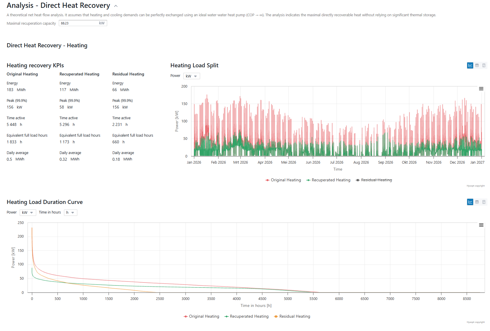
For this analysis, perfect heat exchange is assumed, where heating energy and cooling energy can be exchanged freely. While this does not represent a real system, it provides insight into the maximum theoretical recovery potential.

The analysis is presented from two complementary perspectives.

Heating Perspective

From the heating perspective, the heating demand is split into:

• Original heating demand, as obtained from the general load analysis

• Recuperated heating, representing heating that could theoretically be covered from the cooling energy. The curve equals the recuperated cooling curve in the cooling section.

• Residual heating demand, which remains after maximum theoretical recovery

• Maximum recuperation capacity, this input parameter defines the desired recuperation capacity. Adjusting it will automatically update the residual heating, recuperation, and residual cooling charts and values to reflect this design choice.

• 

  

  
  

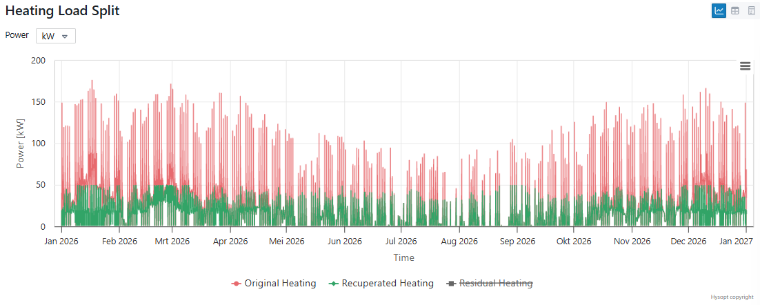
Key performance indicators and load duration curves are provided for these components. In particular, the load duration curve of the recuperated heating can be used to identify a sensible size for a potential heat recovery unit.

Cooling Perspective

The cooling perspective applies the same logic to cooling demand. Cooling demand is split into original, recuperated, and residual components.

Due to the idealised assumption of perfect exchangeability, the recuperated cooling profile mirrors the recuperated heating profile. This symmetry helps support sizing considerations from both perspectives.

Cumulative Heat Balance

The final section of the Simulation Dashboard shows the cumulative heat balance over time. This curve integrates the difference between heating and cooling demand and visualises how this balance evolves throughout the simulation period. The cumulative heat balance section focuses on the balance between heating and cooling energy over the year and can be used for analysing potential for heat recovery via storage systems.

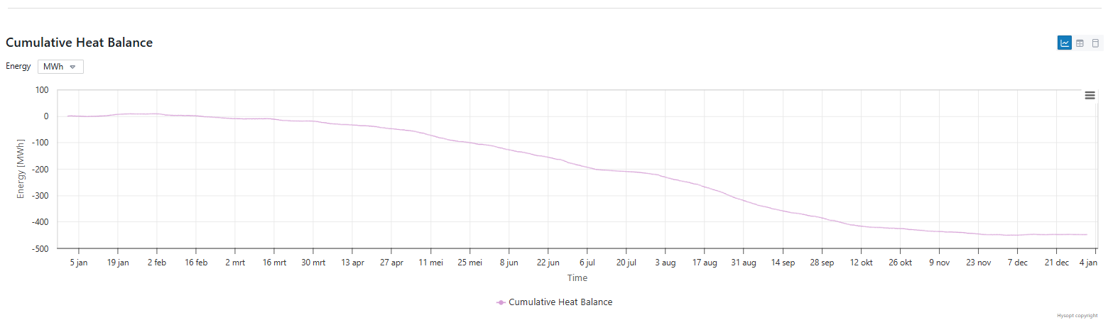
The cumulative heat balance is primarily used to assess the potential effectiveness of thermal storage systems:

• Long-term or seasonal oscillations suggest potential for seasonal storage.

• Short-term oscillations indicate potential for short-term storage

• Limited variation suggests that direct heat recovery is likely more effective than storage if present

Because storage systems inherently introduce losses, this section helps determine whether storage is likely to add value compared to direct heat recovery.

For an elaborated example on how to interpret the Hysopt Simulation Dashboard, see Hysopt Simulation Dashboard – Example Load Profile Analysis