Radiators and convectors are end units that transfer heat toward their environment by radiation & convection. They represent end units within the model, meaning that no BCs can be placed further downstream as they have no secondary gate.
Radiator/Convector end units are in most cases expected to be assigned to a zone. For more information about zone assignment, consult Zone library | Assign base circuits and pipes to a zone .
Radiator/Convector types
At the moment, the Hysopt Optimiser supports five different radiator/convector BC types.
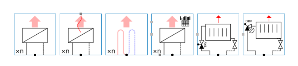
Radiator/Convector
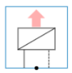
The basic BC representing a heat emitting system. It has various uses:
-
Group of heat emitters: In conceptual analysis, the ‘radiator/convector’ BC can be used to represent a group of heat emitters (typically radiators, radiant panels or fan coil units). By grouping emitters into one BC (instead of modeling each emitter system by its own BC), the Optimiser will require much less calculation time, which will shorten simulation times.
-
Heating battery: In conceptual analysis, the ‘radiator/convector’ BC can be used to represent a heating battery, generally installed within Air Handling Unit (AHU) systems (typically frost batteries, pre-heating batteries or re-heating batteries). Those batteries could also be grouped to reduce the simulation times.
-
Single radiator/convector: In technical/detail analysis, the ‘radiator/convector’ BC can be used to represent a single emitter. This will be necessary to calculate all power propagations and all pressure drops within the model accurately.
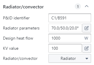
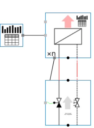
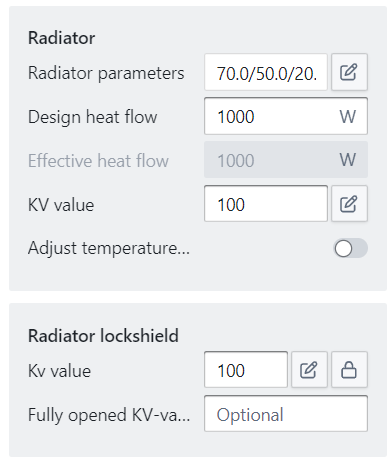
The ‘radiator/convector’ BC is a simple end unit circuit as it has no control & balance valve components. It only regards the emitter as a component. It has the following parameters:
Radiator parameters: The designed temperature regime of the emitter. This must be manually filled in by the user, as its value will affect the design flow rates that will be propagated upstream during the ‘compute design flows’ step. By default, the temperature regime is set at 70/50 °C at an environment temperature of 20 °C for the ‘radiator/convector’ BC and at 30/23 °C at an environment temperature of 20 °C for the ‘floor heating loop’ BC.
Design heat flow: The installed heat emission capacity. This must be manually filled in by the user, as its value will affect the design flow rates that will be propagated upstream during the ‘compute design flows’ step. By default, this value is set at 1 kW.
KV value: The KV value expresses the amount of flow for a pressure drop of 1 bar. This must be manually filled in by the user, as its value will affect the pressure drop propagated upstream during the ‘optimise components’ step. By default, this value is set at 100.
If the actual KV value isn't known, the user can click on the "pencil" icon which results in a calculation popup window. In the popup window, the user can calculate the KV value by entering the pressure drop and flow rate (and if needed, the brine, mixture and reference temperature). This option is preferred when the information on the boiler is known. However, the user can also let the software automatically calculate the KV value depending on the design flow rate by using the other tab and entering the estimated pressure drop over the radiator.
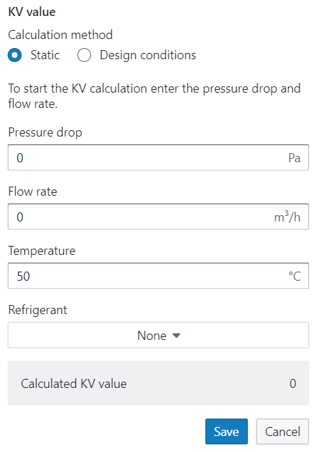
Important: Don’t forget to save the calculated KV value. If you click somewhere else in the model before saving, the calculation will be canceled.
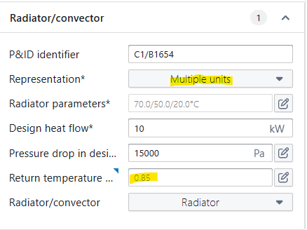
Representation* and return temperature behaviour factor
For the representation parameter, there are two possible settings:
-
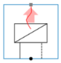
Single Unit: This BC represents 1 end unit (e.g. 1 radiator or 1 convector)
-
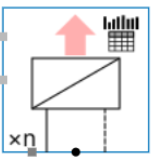
Multiple units: This BC is a combination of multiple end units. e.g. an equivalent unit representing an entire circuit of radiators. Often used in conceptual models, where the full installation is not drawn in detail.
This distinction is very important for the return temperatures during dynamic simulation. The average combined return temperature will depend heavily on the number of active units and the load of these units.
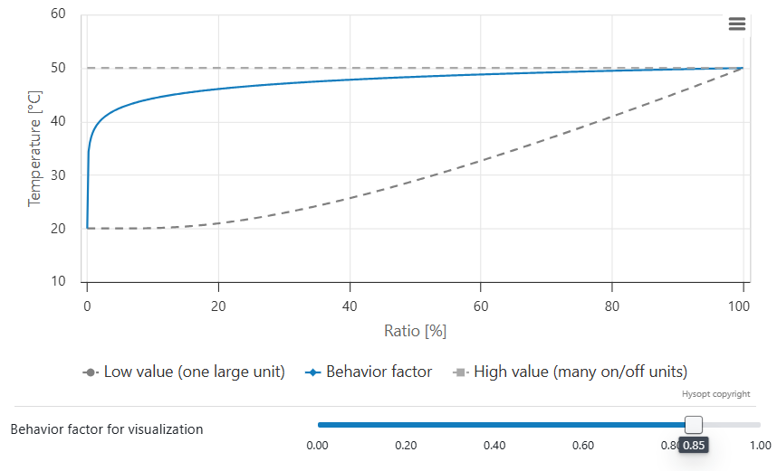
The return temperature behaviour factor allows you to calibrate the return temperature of an equivalent end unit circuit to measurement data. If no measurement data is available, Hysopt advises a default setting of 0.85 based on historical measurement data.
You can further tweak the return temperature behaviour using following trends:
Lower value
-
The system behaves more as one large end unit.
-
Individual end units tend to be active mostly at the exact same time.
-
At partial load, return temperatures closer to the environment temperature are expected.
Heating
At partial load, lower return temperatures are expected.
Cooling
At partial load, higher return temperatures are expected.
Higher value
-
The system behaves more as many end units.
-
Individual end units tend more towards on/off behaviour.
-
At partial load, return temperatures closer to design return temperature are expected.
Heating
At partial load, higher return temperatures are expected.
Cooling
At partial load, lower return temperatures are expected
Context
The return temperature is a crucial parameter in the design and performance of energy systems. When multiple end units (e.g. radiators) are represented as a single equivalent end unit, abstraction is made from the state of each individual end unit. This introduces uncertainty in the predicted return temperature at partial load.
Example
Consider a system with:
-
Number of radiators: 100 units
-
Power per radiator: 1 kW (≈ 3.41 MBH)
-
Design heat flow: 100 kW (341 MBH)
-
Design regime: 70/50/20 °C (158/122/68 °F)
-
Actual supply temperature: 70 °C (158 °F)
-
Actual zone temperature: 20 °C (68 °F)
-
Actual heat flow: 15 kW (51 MBH)
There are two edge cases that can deliver this 15 kW:
-
Many radiators active at low flow rate
-
Water flows slowly through each element.
-
Return temperature approaches the zone temperature (~20 °C / 68 °F).
-
-
Few radiators active at design flow rate (the rest switched off)
-
A few radiators each deliver a larger share of the total power.
-
Return temperature approaches the design return temperature (~50 °C / 122 °F).
-
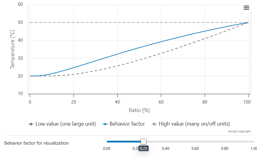
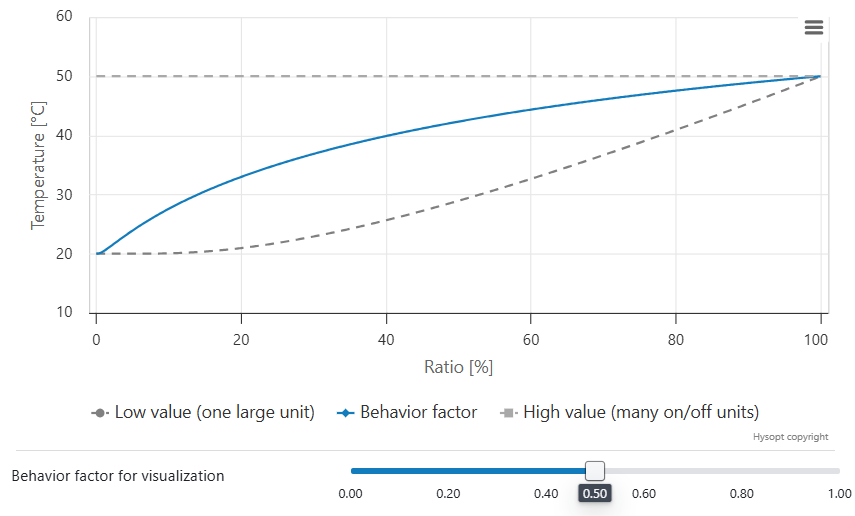
Conclusion
A return temperature between approximately 20 °C (68 °F) and 50 °C (122 °F) is physically possible, depending on the activation state of the individual end units. The return temperature behaviour factor governs how the model transitions between these limits as the load varies. When measurement data is available, this factor should be calibrated accordingly; otherwise, the recommended default value of 0.85 can be applied as a conservative assumption. The resulting behaviour is illustrated in the charts below for three example cases.
Radiator/convector: A drop down list in which the user can specify if the BC represents a radiator or a convector. The selection will somewhat alter the heat flow calculation, as it changes the exponent nrad within the emitter model. See above for a more detailed explanation of the model’s formulas.
By default, the BC is set to represent a radiator.
The ‘radiator/convector’ BC (in contrast to the ‘dynamic radiator without zone’ BC, see below) must always be assigned to a zone to properly simulate the model. It is therefore mainly used to represent heat emitting groups within rooms where the room temperature is controlled. More information on the control strategy of a room controller can be found here: Modulating room controller for heating/cooling (Thermostat).
Dynamic radiator without zone
From a modeling point of view, this BC is completely similar to the ‘radiator/convector’ BC. Its only difference lies within the control strategy. The previous BC must always be assigned to a zone to properly simulate the model. If no such zone is available, or if the zonal control model is not applicable, this BC must be used. A specific control strategy for the design load must subsequently be made by the user instead.
This BC is most commonly used to model heating batteries, especially for those within Air Handling Units (AHU). As the Optimiser currently does not regard calculations at the air side of the AHU, a specific control strategy is set up to correctly estimate the heating battery’s heat load. A further explanation of how to implement AHUs correctly in the Optimiser can be found here: Capacity controlled Air Handling Units.
Radiator with heat flow control
This BC can be used to directly link building energy modelling thermal load data to the equivalent end-unit block in Hysopt. This BC has internal load control, where the output connection can be used to control the load output of this radiator BC. The 2 available input connections are:
-
Activation Signal
-
Desired Heat Flow
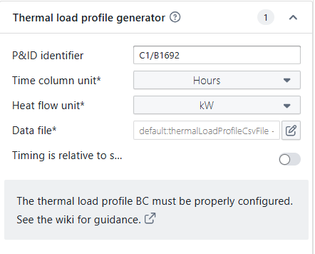
Example:
Connect the thermal load profile generator to the radiator with heat flow control. Ensure that the CSV input file is adapted to the project-specific thermal load to which this end unit is subjected. More guidance on csv file handling: Data files
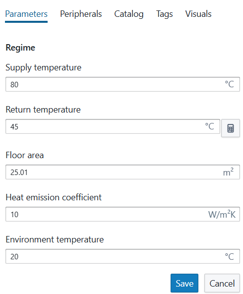
Floor heating loop
This BC can be used to represent floor heating circuits in the model. However, from a modeling point of view, this BC is completely similar to the ‘radiator/convector’ BC.
When clicking the temperature regime of an underfloor heating, you will see an additional calculator option.. This calculator allows you to calculate the return temperature from your underfloor heating system using the supply temperature, environment temperature, floor area and heat emission coefficient as input. The calculation is based on the UA*LMTD, with U the heat emission coefficient of the floor area (W/(m²K)), A the floor area and LMTD the logarithmic mean temperature difference between the water and the environment.
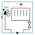
Radiator with thermostatic radiator valve
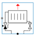
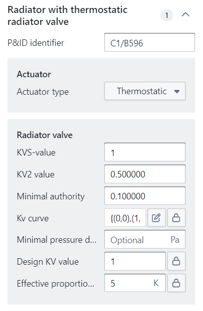
This more advanced BC represents a heat emitting system along with its control & balance valve components. It represents a single radiator that is controlled by a thermostatic valve and is mainly used in technical/detail analysis.
The BC itself does not have any parameters, but it encompasses different components:
-
Radiator valve: A two way control valve with a detailed list of parameters to correctly compute the flows & pressure drops. A more detailed description of its parameters can be found here:
Control valves | Radiator valve. -
Radiator: The emitting end unit with the same parameters as the ‘radiator/convector' BC (see above).
-
Radiator lockshield: A two way balance valve that is typically placed at the complete other side of the radiator valve. In theory, the lockshield is used to balance your radiator circuit. In practice, this is not often the case. Lockshield valves are usually set on a default value while being placed. Therefore, as a rule of thumb, the pressure drop over the lockshield valve can be estimated by filling in a KV value of 2.5.
Radiator with dynamic radiator valve
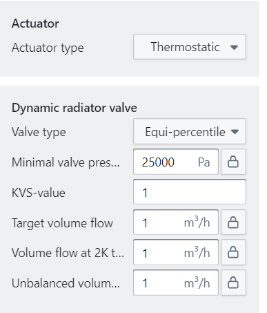
This BC is similar to the ‘radiator with thermostatic radiator valve’ BC, with the exception that the thermostatic radiator valve is replaced by a dynamic radiator valve. It has, therefore, the same parameters as a pressure independent control valve (see Balance valves | Pressure independent control valve), with the addition of the parameter ‘Volume flow at 2K temperature error’ which sets a target volume flow when the actual temperature is 2 °C away from its design point.
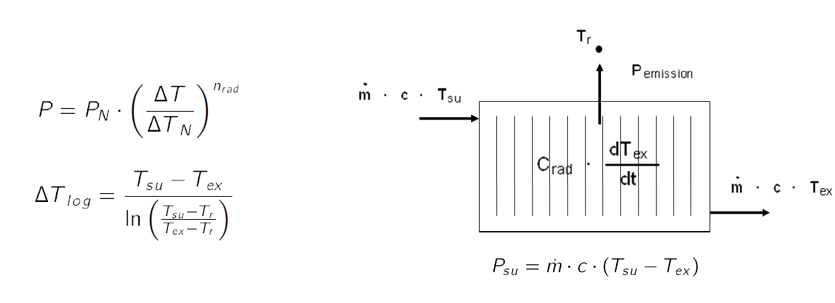
Radiator Model
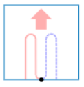
To study the radiator dynamics and to analyze the respective influence on the overall system behavior, a dynamic radiator model is required. When considering the radiator from an Eulerian perspective, the radiator dynamics can be modeled according to a dynamic heat balance in which the lumped thermal capacitance is assumed to be concentrated in the exhaust temperature node.
Psu is the thermal power supplied to the radiator and equals the net difference between the incoming and leaving heat flows as illustrated in the figure below. The heat emission Pemission is described using the exponential relationship between the radiator performance and the logarithmic mean temperature difference according to the 2 equations below. The exhaust temperature of the radiator changes according to the supplied thermal power and the heat emission. The exponent nrad in the equation below determines the characteristic of the used end-unit. In the case of a radiator, it is (1,2 ... 1,34) and a convector (1,25 ... 1,45).