The pipe heatmap provides a visual overlay on HVAC schematics, using color-coding based on multiple selectable parameters to deliver deeper insights.
Since some parameters are pressure-drop related, it is important that the pipe selection and optimise component step were completed.
Usage: Activation of the pipe heatmap


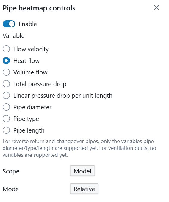
Press the pencil button in the top ribbon bar to open the pipe heatmap menu, which appears as as sidebar at the right-hand side. In the pipe heatmap menu, you will find all settings for the pipe heatmap. To get started, you first need to enable the pipe heatmap to the current model.

Enable the heatmap manually using the toggle. When activated, additional parameters appear below the toggle, allowing you to choose which values you want to analyse. Beneath these parameters, you will find two extra settings that define the scope of the pipe heatmap and the view mode.
The view mode can be set to either Relative or Absolute. In Relative mode, the maximum and minimum recorded values in the model are used as the scaling limits. In absolute mode, the user can provide the limit values manually.
The Scope setting is only relevant when the view mode is set to Relative. When the scope is set to Model, the minimum and maximum values used as scaling limits are determined across the entire model. This ensures a consistent legend over all canvases. To analyse differences on a single canvas, you can switch the scope to Canvas. In this case, the scaling limits are based only on the active canvas. Each canvas will then have its own legend, making it easier to investigate local differences in detail.
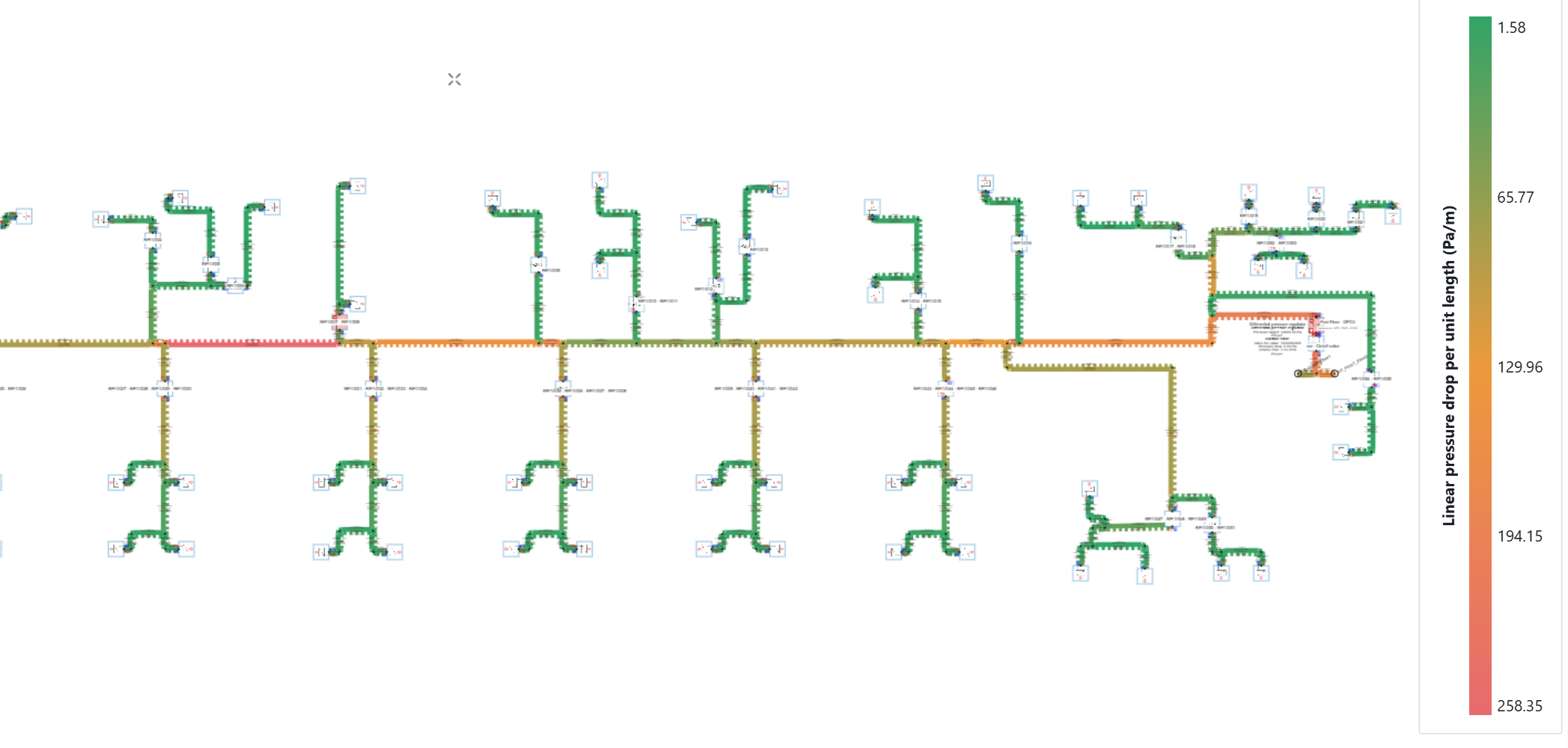
Application example 1: investigation of possible future extensions on an existing HVAC model.
In a detailed Hysopt model, the pressure drop per meter parameter was selected to evaluate the pressure loss per unit length across all pipes. The color coding immediately highlights potential bottleneck pipes for future integration of additional units.
The red pipes indicate pipes with high pressure drop per meter. adding a new radiator will increase the flow across that pipe and in turn, will increase the pressure drop per unit length.
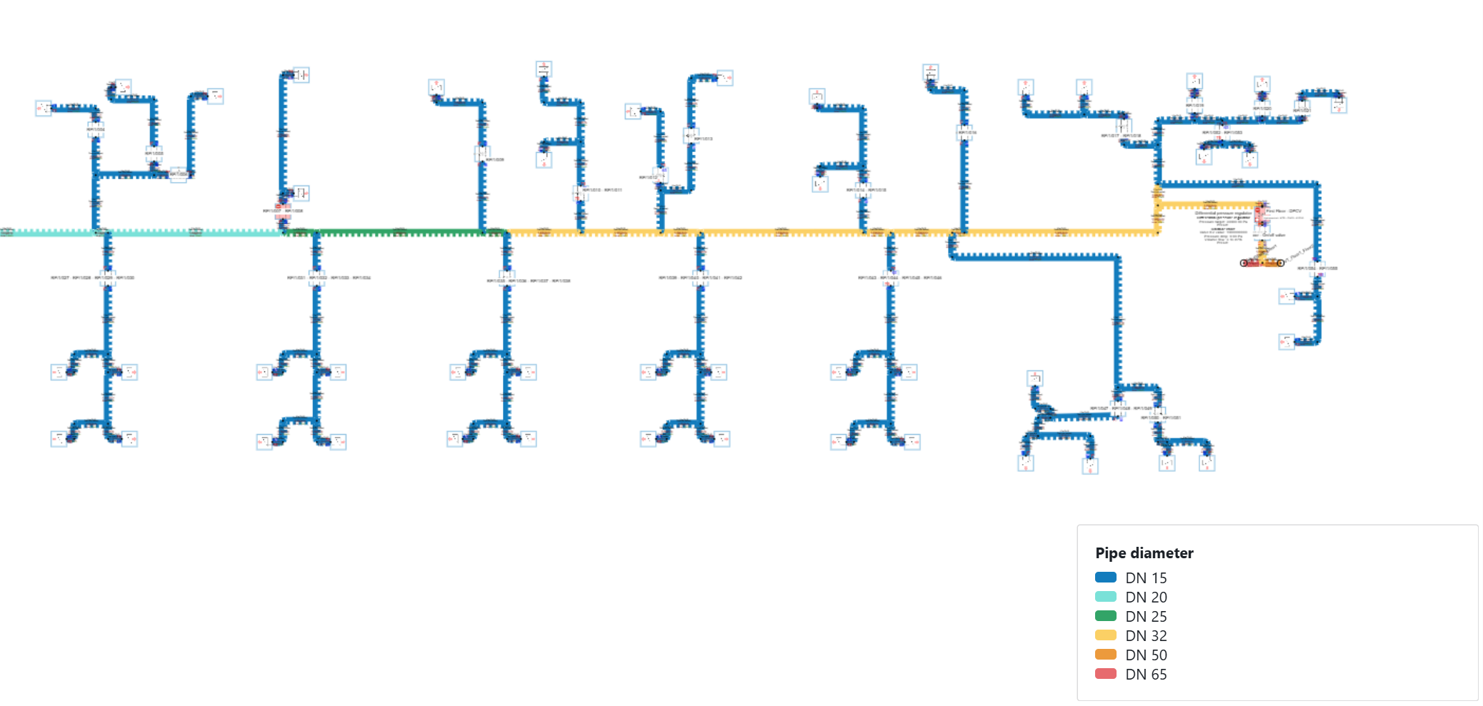
Application example 2: Visual representation of the installed pipe diameters.
This visual check clearly shows that the main distribution branch has a decreasing pipe size from the main riser, while all ancillary branches use a DN 15 pipe size.
Can be valuable in combination with the PDF exports for technicians on-site who have to install the pipework.