Hysopt Simulation Dashboard – Example Load Profile Analysis

1. Introduction

This page demonstrates how the Hysopt Simulation Dashboard can be used to analyse heating and cooling load behaviour and to extract design‑relevant insights at an early stage of HVAC system design. Two different heating and cooling load profiles are evaluated using the same simulation model.

2. Model Description and Assumptions

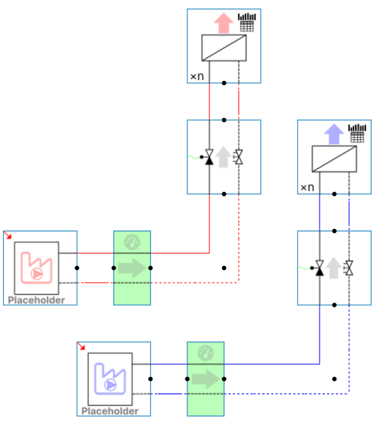
A simple model is created to perform the Hysopt simulation. Dashboard metering base circuits are used to capture the simulated heating & cooling loads that are imposed at the end units. For both profiles, the installed heating and cooling capacities are 65 kW.

As this analysis focuses on the load profiles, the primary side remains out of scope. The energy producers are therefore replaced by generic production units.

3. General Load Analysis

3.1 Profile 1 – Heat Flow Behaviour

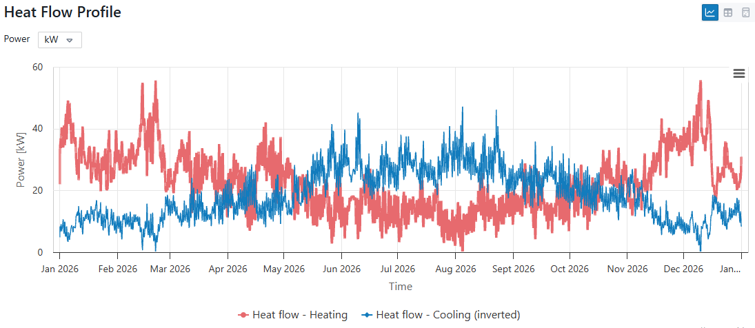
Profile 1 is characterised by continuous heating and cooling demand throughout the year. Both services remain active for almost the full simulation period, indicating stable base loads and a high degree of simultaneity.

3.2 Profile 2 – Heat Flow Behaviour

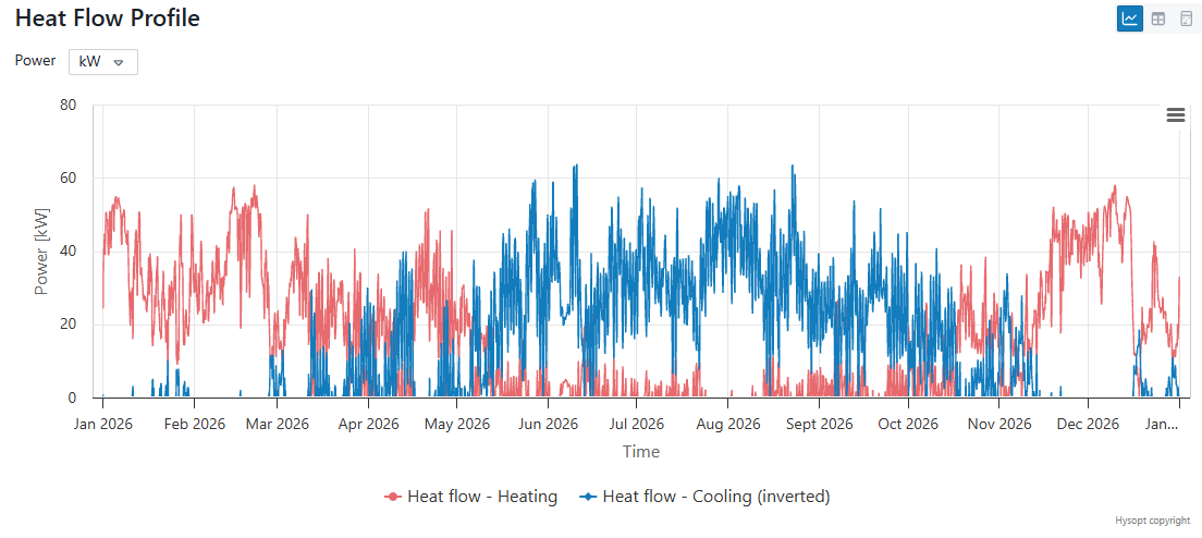
Profile 2 shows a strong seasonal behaviour. Heating demand is mainly present during winter, while cooling demand is concentrated in summer, indicating a low degree of simultaneity.

3.3. Key Performance Indicators

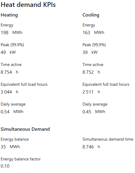
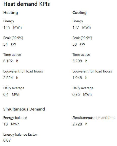
The KPI overview highlights clear differences between both profiles. Profile 1 has higher annual heating and cooling energy demand and significantly longer activation times, while Profile 2 has higher peak loads despite lower total energy use.

Profile 1 also shows higher equivalent full load hours, indicating it makes more intensive use of its installed capacity. Profile 2 shows lower equivalent full load hours, indicating its installation is more driven by short, high-intensity peaks.

The energy balance factor is slightly closer to zero for Profile 2, indicating a more balanced annual energy split, what will be beneficial for long term storage. Profile 1 shows substantially longer periods of simultaneous demand, which is better suited for direct heat recovery.

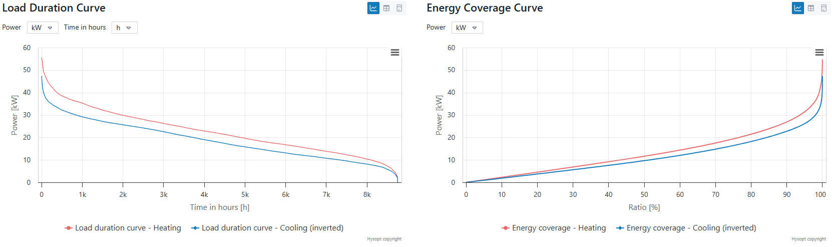
3.4 Load Duration Curves & Energy Coverage Analysis

Note that loads for heating and cooling are sorted independently: identical durations do not imply coincidence in time.

Profile 1

Profile 2

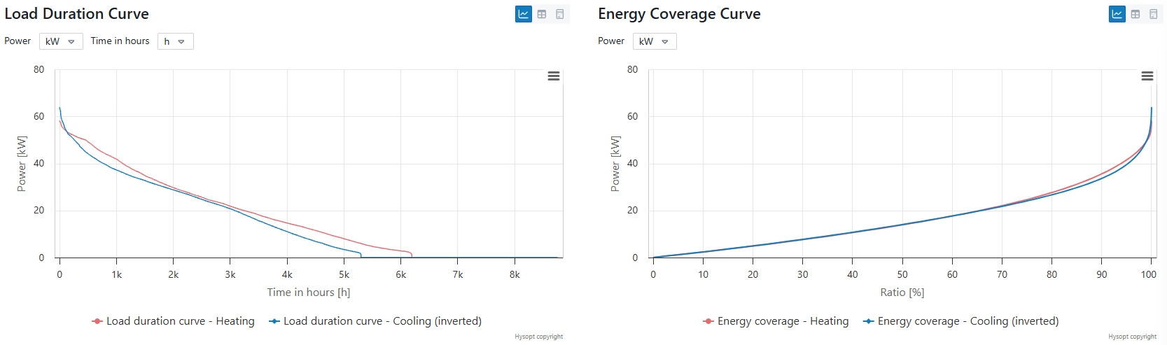
Load Duration Curves

The Load Duration Curve for profile 1 almost spans the entire year and shows that the system continuously operates in partial load conditions. For profile 2, the load durations are significantly shorter, indicating that heating and cooling loads are concentrated in distinct periods.

Energy Coverage Curves

The Energy Coverage Curves illustrate how much of the annual energy demand can be supplied by a given capacity. For profile 1, 80% of the heating & cooling energy is can be covered by a heating & cooling source with a capacity of ~ 20 kW. For profile 2, a heating & cooling capacity of ~ 27 kW is required to cover 80% of the energy demand. Remember that both profiles have an installed heating & cooling end unit capacity of 65 kW. This demonstrates that relatively small base‑load sources can already cover a large share of total demand, highlighting opportunities for hybrid system concepts.

3.5. Monthly Energy Distribution

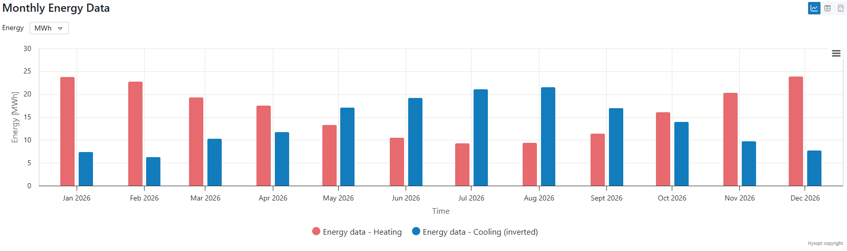
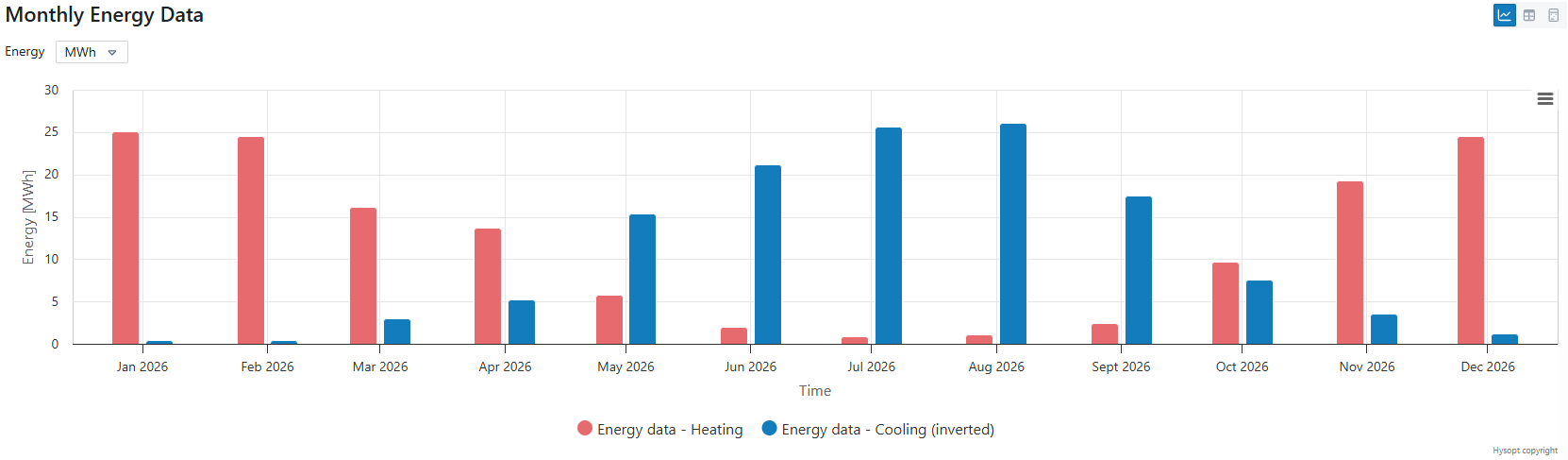
The Monthly Energy Data further illustrates the contrast between the profiles. Profile 1 shows a relatively even distribution of heating and cooling energy throughout the year. Profile 2 shows heating energy concentrated in winter months and cooling energy concentrated in summer months, limiting the (direct) heat recovery potential.

4. Direct Heat Recovery Analysis

For direct heat recovery, no thermal storage is considered. Perfect heat exchange is assumed to illustrate the maximum theoretical recovery potential.

4.1 Heating Perspective

From a heating perspective, recovery occurs when cooling demand is available simultaneously.

Profile 1

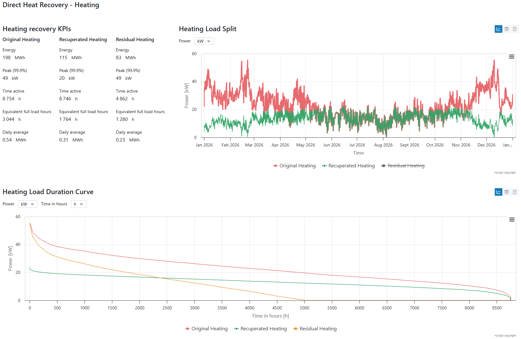
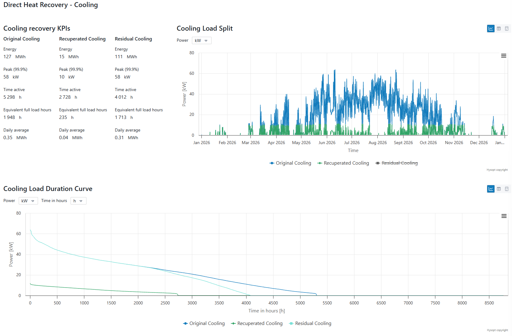
The Heat Load Split graph illustrates when heat is recuperated from the cooling profile. Profile 1 shows strong recovery potential, as a significant share of the annual heating demand can be recuperated from cooling, with recovery possible during almost the entire year.

The heating recovery KPIs highlight the potential for heat recuperation from the cooling profile. Most of the heat demand can be recovered from the cooling demand. However, the peak recovery capacity is 20 kW, much lower than the peak demand of 49 kW. The peak recovery capacity is an important number, as it highlights the maximal useful size for the recuperation unit.

While heat recovery drastically reduces the residual annual heating energy, the residual heating source must still be designed based on the full peak heating capacity. This indicates that the heating peak demand occurs during moments without cooling demand.

The Load Duration Curves visualise the impact of heat recuperation on the heating demand. Through heat recuperation, a base load of maximal 20 kW can be provided for the heat demand throughout the year. A residual heat source with a capacity equal to the peak demand will be required for ~ 5000 hours per year.

Profile 2

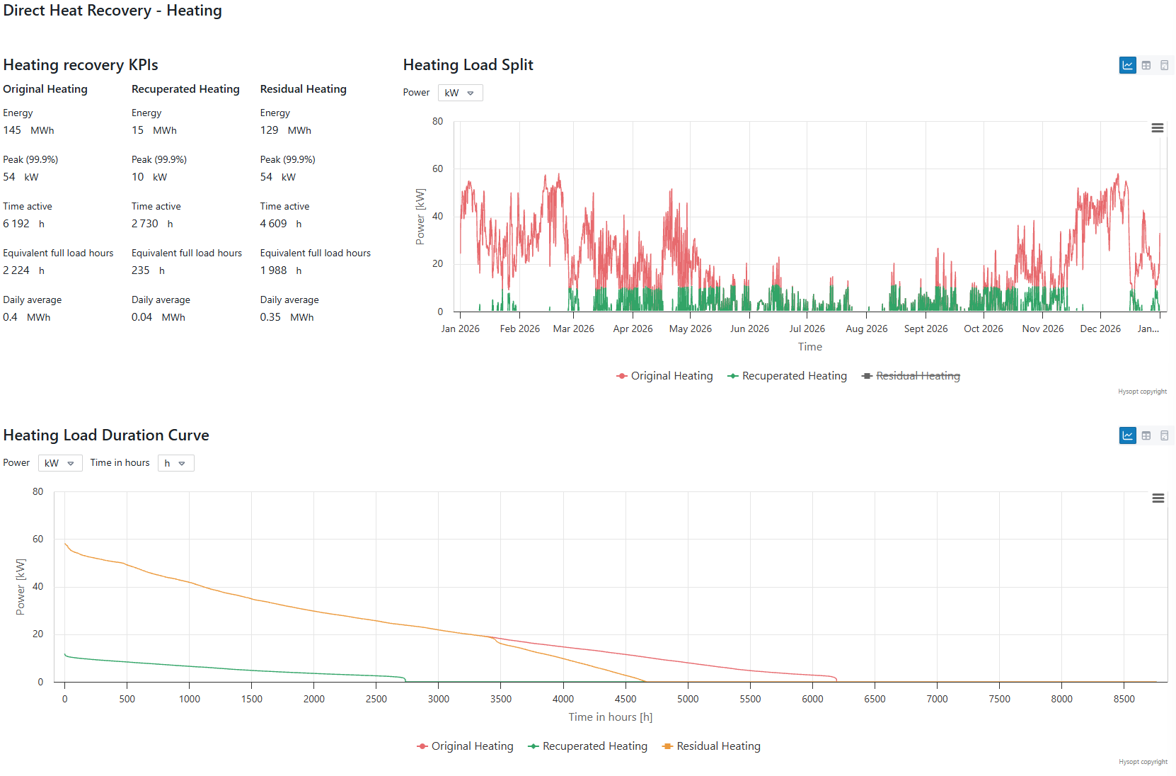
Looking at the Heat Load Split graph & the Load Duration Curves for profile 2, the potential for heating recovery is limited. Recovery mainly occurs during summer, while almost no recuperation is possible in winter when heating demand peaks. The KPIs further confirm this, with a peak recovery capacity of 10 kW and only ~ 2700 recovery hours per year. The residual heating source again must be designed to the full peak heating capacity.

4.2 Cooling Perspective

From a cooling perspective, recovery occurs when heating demand is available simultaneously.

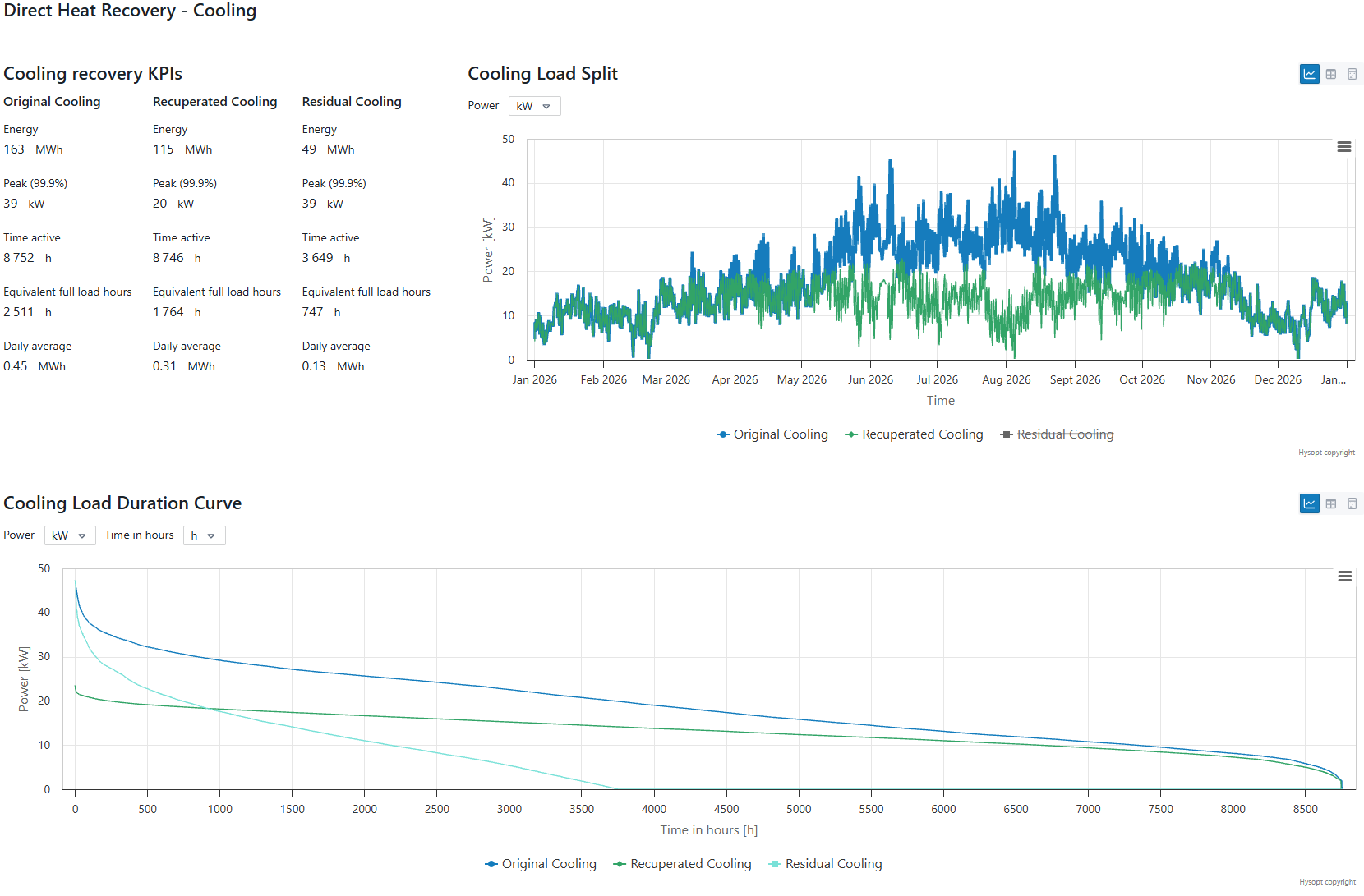
The same analysis can be made from a cooling perspective. Profile 1 shows a strong simultaneity with the same base load of maximal 20 kW recovered energy. Profile 2 has limited recovery potential, with a maximal peak recovery of 10 kW and only ~ 2700 recovery hours. Both profiles require a residual cooling source, designed based on the full peak cooling capacity.

Profile 1

Profile 2

5. Cumulative Heat Balance

When (long term) thermal storage is considered, the cumulative heat balance provides insight into the seasonal mismatch between heating and cooling energy and allows an assessment of how effectively long‑term (seasonal) thermal storage could be used to improve system performance.

5.1 Interpretation of the Cumulative Heat Balance

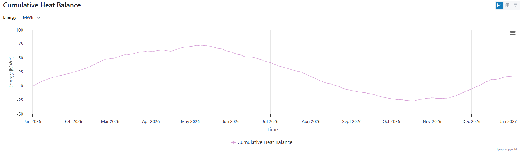
The cumulative heat balance represents the time‑integrated difference between heating demand and cooling demand. A positive slope indicates a period where heating demand exceeds cooling demand, a negative slope indicates a period where cooling demand exceeds heating demand. The absolute value represents the amount of excess thermal energy that could potentially be stored or must alternatively be rejected

Typically, the cumulative heat balance for heating & cooling systems follows a wave pattern where the imbalance steeply increases in winter due to high heating demand combined with low cooling demand, and steeply decreases in summer due to low heating demand combined with high cooling demand. In spring & autumn, the slopes decrease, flatten out, and invert as the dominance between heating & cooling demand inverts.

5.2 Cumulative Heat Balance – Profile 1

For profile 1, the cumulative heat balance shows a continuous positive surplus, originating from the excess recoverable cooling energy during the winter months, with a maximum imbalance of approximately 50 MWh at the beginning of summer. The imbalance gradually decreases during summer as cooling demands becomes dominant.

This behaviour indicates that seasonal thermal storage could be highly effective, allowing excess cooling energy recovered in winter to be stored and reused during summer. However, at the end of the year, a residual imbalance of 35 MWh remains. To avoid this surplus to build-up over the years, an energy dump is required.

5.2 Cumulative Heat Balance – Profile 2

For profile 2, the cumulative heat balance behaves differently, as the imbalance becomes negative towards the end of the summer, indicating that the cumulated cooling demand exceeds the cumulated heating demand at that period. The maximum imbalance reaches 70 MWh at the beginning of the summer, before its decreases to a peak of -25 MWh in autumn, after which it gradually recovers towards the end of the year, ending with a surplus of 18 MWh, which is significantly smaller than for Profile 1.

Despite the higher maximum imbalance, profile 2 shows a better long‑term seasonal closure. This makes it better suited for integration with seasonal thermal storage, as the excess energy is more effectively balanced over the year, and the need for permanent energy dumping is reduced.

6. Conclusions and Design Implications

6.1 Summary of the Hysopt Simulation Dashboard Analysis

The Hysopt Simulation Dashboard was used to analyse two distinct heating and cooling load profiles and to assess their implications for system design, capacity sizing, and heat recovery potential.

The general load analysis demonstrated fundamentally different load behaviours:

• Profile 1 exhibits a high degree of simultaneity between heating and cooling demand throughout the year. Although seasonal trends are still present, both loads remain active almost continuously, with the system operating entirely in partial load regimes.

• Profile 2 shows strongly time‑separated heating and cooling demands. Loads are concentrated in specific periods, resulting in limited simultaneity and shorter overall activation times.

The direct heat recovery analysis further highlighted the contrast between both profiles:

• For profile 1, a near‑continuous base load exists where heat can be recovered from the cooling demand. The analysis showed a maximum recoverable capacity of 20 kW, which defines the upper limit for the useful size of a heat recovery unit.
  This recoverable capacity is significantly lower than:

  • The peak heating demand (49 kW)

  • The peak cooling demand (39 kW)

  • The installed end‑unit capacities (65 kW)

  Consequently, even with optimal heat recovery, residual sources are required, sized to the full peak demand.

• For profile 2, the potential for direct heat recovery is very limited due to minimal overlap between heating and cooling demand. Heat recovery contributes only marginally to the total energy demand, and the system remains primarily dependent on its residual heating and cooling sources, which must again be sized to peak demand.

The cumulative heat balance analysis provided additional insight from a seasonal perspective:

• Profile 1 shows a seasonal trend with a net positive annual surplus. Seasonal storage can be effective, but only if combined with an energy dump mechanism to prevent long‑term accumulation.

• Profile 2 presents a more balanced cumulative heat profile over the year. Despite larger peak imbalances, the final annual imbalance is small, making this profile better suited for systems with seasonal thermal storage without necessarily requiring continuous energy dumping.

6.2. Next steps in design choices

As such, the capacity values proposed below should be regarded as first‑order design magnitudes. Once a preferred system concept has been selected, further optimisation can be performed by running sensitivity analyses in Hysopt, refining heat pump sizes and operational strategies.

Based on the findings, the following design directions can be considered.

6.3 Design implications for profile 1

Direct Heat Recovery–Driven Concept

The high simultaneity between heating and cooling demand makes profile 1 well suited for systems that directly utilise heat recovery, such as a 4‑pipe water‑water heat pump.

A first‑order sizing follows directly from the maximum recoverable heat capacity:

• 1 × 4‑pipe water‑water heat pump
  Rated 20 kW @ reference temperature conditions

The remaining heating and cooling demand can be covered by a reversible heat pump sized on the residual peak demands:

• 1 × 2‑pipe reversible air‑water heat pump, sized on the most critical condition of:

  • 50 kW @ required heating conditions

  • 40 kW @ required cooling conditions

This configuration maximises direct recovery while maintaining full peak redundancy.

Seasonal Storage–Driven Concept

Due to its seasonal behaviour, Profile 1 is also suitable for seasonal thermal storage solutions, such as ground‑coupled systems combined with a 4‑pipe water‑water heat pump.

In this case, the heat pump can be sized closer to total demand, as excess energy can be stored:

• 1 × 4‑pipe water‑water heat pump
  Rated 50 kW @ reference temperature conditions

• Ground system, sized to:

  • Extract 50 MWh of heat annually

  • Deliver 40 kW of cooling @ reference temperature conditions

• Dry cooler, sized to:

  • regenerate 35 MW of heat annually

  • Operate below 40 kW to remain compatible with the ground system

The dry cooler is required to manage the net positive cumulative heat balance and prevent long‑term thermal drift.

Alternative hybrid configurations are also possible. Note that every design choice also has an investment cost, which is out of scope for this analysis.

6.4 Design implications for profile 2

Seasonal Storage–Driven Concept

Due to its limited simultaneity, profile 2 is not suited for systems relying on direct heat recovery. However, its strong seasonal complementarity makes it highly attractive for solutions with seasonal thermal storage.

A first‑order concept is:

• 1 × 4‑pipe water‑water heat pump
  Rated 60 kW @ reference temperature conditions

• Ground system, sized to:

  • Extract 70 MWh of heat

  • Store 25 MWh of heat

  • Deliver 60 kW of cooling @ reference temperature conditions

In a first design iteration, no heat dump is included. Further simulations should determine whether long‑term imbalance necessitates the addition of a dry cooler.

Peak‑Driven Concept (No Seasonal Storage)

If seasonal storage is not feasible, a 4‑pipe water‑water heat pump is not advised for profile 2. The limited duration and capacity of heat recovery do not justify the investment.

A more suitable approach is to rely on independent production sources:

• 2 × 2‑pipe reversible air‑water heat pumps, sized for the peak conditions for heating & cooling

  • 1 x 55 kW @ required heating conditions

  • 1 x 60 kW @ required cooling conditions

Using reversible units instead of a traditional heat pump‑chiller combination is advantageous, as long periods exist with only heating demand or only cooling demand. During such periods, both units can operate in the same mode, meaning that effective installed capacity may be lower than the individual peak values. Further optimisation of this concept can be achieved by running sizing sensitivities in Hysopt.

6.5 Final Remarks

This study confirms that load simultaneity, seasonal balance, and energy timing are critical parameters in HVAC system design. The Hysopt Simulation Dashboard enables these aspects to be quantified clearly, allowing designers to move beyond peak‑based sizing and towards robust, energy‑efficient system concepts.