Dynamic simulation

Dynamic simulations

The Hysopt software can do dynamic simulations with a time step of 30 seconds. The time step is quite short to allow quick behavior changes in a system (e.g. domestic hot water tapping, quick opening valves, …).

The dynamic simulation in Hysopt has three solvers to allow accurate physical behaviors of a complete system:

Hydraulic solver
Thermal solver
Control solver

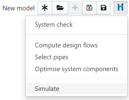
To start the dynamic simulation in Hysopt, the user should click on the “Simulate” button visualised below.

After clicking on the “Simulate” button, a pop-up window appears. In the pop-up window, the user can change the start date, simulation duration, and weather profile.

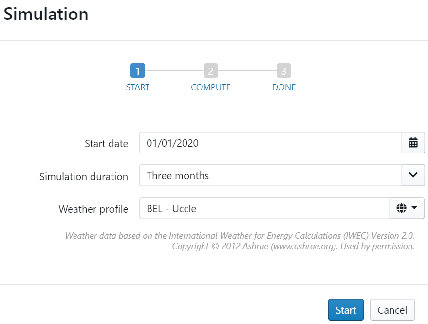
The simulation duration can be up to 20 years, which might be useful when using geothermal energy storage systems. More information about geothermal energy storage systems can be found in Geothermal energy storage templates.

Weather profiles

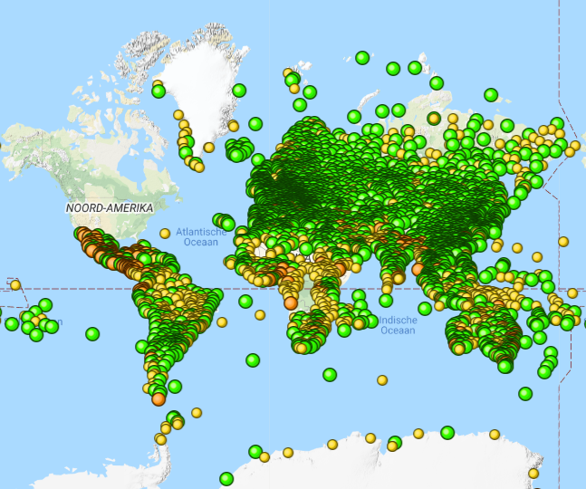
Hysopt supports 3,012 weather profiles in 6 continents and 160 countries, provided by ASHRAE aand Whitebox Technologies. In the following image (green dots) and link, all the locations are visualised. The TYP files are TMY (Typical Meteorological Year) of said locations. More information about a TMY can be found in the Wikipedia link.

http://ashrae.whiteboxtechnologies.com/map-IWEC2

https://en.wikipedia.org/wiki/Typical_meteorological_year

Weather data based on the International Weather for Energy Calculations (IWEC) Version 2.0. Copyright © 2012 Ashrae (http://www.ashrae.org). Canadian weather data based on CN2019. Copyright © 2019 Whitebox Technologies. Used by permission.

Warnings:

“Older” models (before the implementation of the ASHRAE weather profiles) may still use the previously used weather profiles (not from ASHRAE). New models, however, don’t support the previously used weather profiles anymore. The user should make sure he isn’t comparing models with different weather profiles.
When changing the simulation duration, the data interval shown in the graphs change as well. So if the user simulates for one day, the visualised data has a high-resolution meaning quick changes in the behavior of the system are visualised. If the simulation duration is 1 month these quick changes in the behavior aren’t quite as clear anymore because of the larger data interval.
When simulating with a duration larger than 1 month, the transient behavior of the system isn’t visualised anymore because the time interval would be too large to make any correct observations of the system. Integral values of for instance the thermal power is still visualised in some components.

Simulation analysis

After running a dynamic simulation, the results can be analysed directly in the Hysopt model in three ways. You can use the simulation values, use the simulation graphs or use the simulation dashboard.

Simulation values

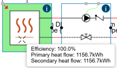
Simulation values are integrated values being displayed as a hover message on base circuits. These parameters are a set of typically relevant parameters to have integrated after a simulation.

You can recognise base circuits with available simulation values by the Info icon . To display them, simple hover with your mouse over the corresponding base circuit.

Simulation values are a limited set of values which might not yield sufficient level of detail for your application. For a more profound analysis of your system and its behaviour, you can use the Simulation graphs and the Simulation dashboard, elaborated below.

Simulation graphs

Simulation graphs can be used to analyse the dynamic behaviour of selected base circuits over the full length of the simulation horizon.

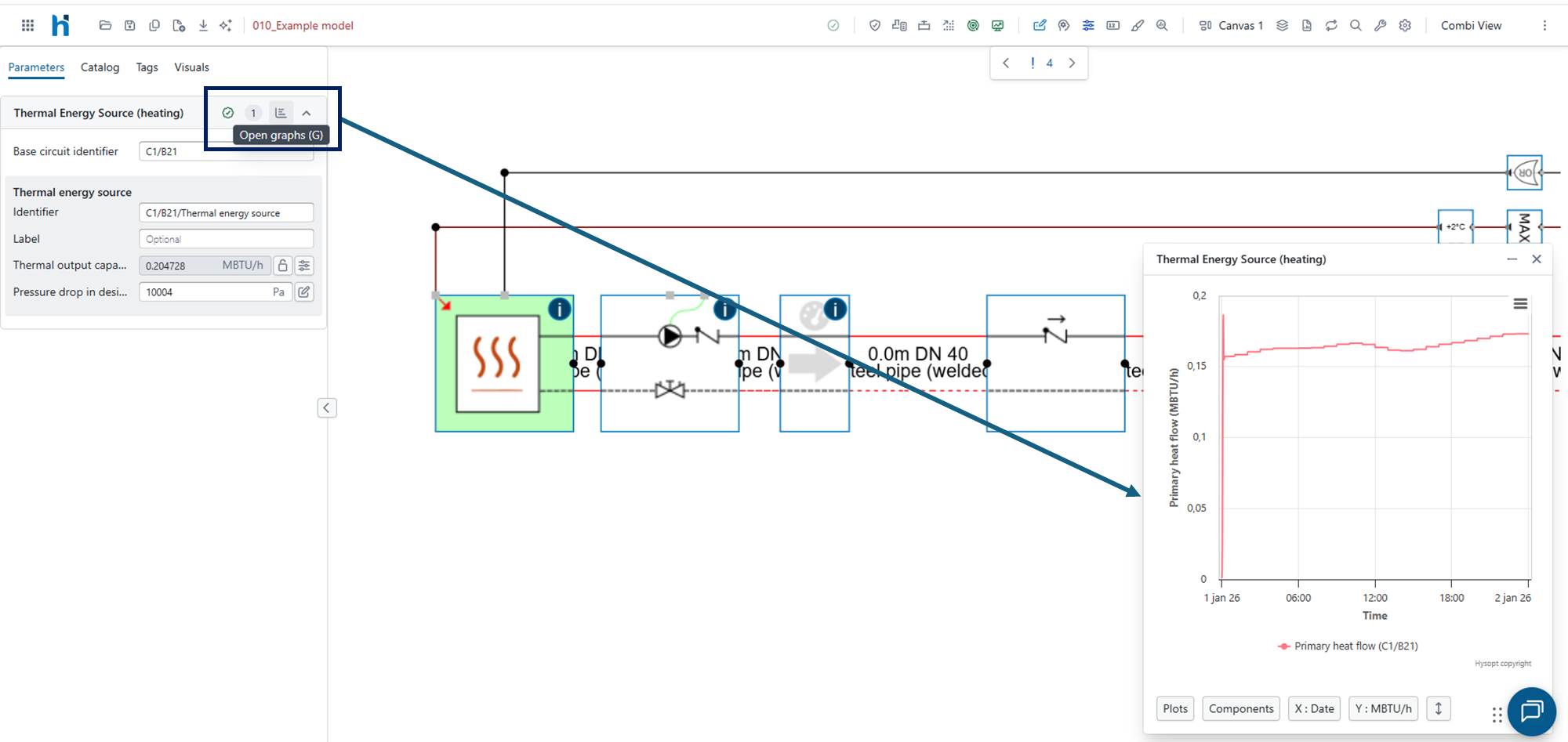
To open a graph, select one or more base circuits and click Open Graphs in the selection toolbar. Alternatively, use the hotkey “G” on the keyboard. When clicking the open graph button, the graphs will open in a pop-up window on the bottom right-corner of the canvas.

In the graph window, the user can choose which simulation parameters to visualise using the “Plots” dropdown in the bottom-left corner. The units and components can also be selected at the bottom of the graph.

The graph supports the following actions:

Action	How to use it
Zoom	You can zoom on the charts by using a zoom box. click and hold+drag over a specific area of the graph to zoom in on that part of the graph. To zoom out, you can use the button
Pan	After zooming in, hold Shift and drag with the left mouse button to move through the graph while keeping the same zoom level.
Reset zoom	Click Reset zoom to return to the original graph view.
Plots	Use the parameter list in the bottom-left corner to enable or disable the results shown in the graph.
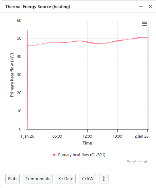
Select units	Use the unit selector at the bottom of the graph.
Toggle graph line	Click an object in the graph legend to hide or show the corresponding graph line. This makes it easier to focus on specific results without changing the selected parameters.
Move graph window	Drag the graph window to another position in the Hysopt environment by dragging the top ribbon bar of the pop-up.
Resize graph window	Drag the edges or corners of the graph window to make it larger or smaller.
Overlay graphs	Open multiple graphs and drag one graph window onto another. Hysopt combines them into one graph, allowing results from multiple base circuits to be compared. You can also overlay graphs by first selecting multiple base circuits and using the hotkey “G”
Export options	Open the graph menu in the top-right corner. From there, you can view the graph in full screen, print it or download it. You can also export the graph data by downloading the data as CSV, or copy the data to the clipboard.

Simulation dashboard

The Hysopt software also provides a pre-built energy analysis tool for your system in the shape of the simulation dashboard. For more information on the usage of the simulation dashboard and explanation on its content, please consult: Simulation Dashboard or Hysopt Simulation Dashboard – Example Load Profile Analysis